BAYESIAN OPTIMIZATION OF CRYSTALLIZATION PROCESSES TO GUARANTEE END-USE PRODUCT PROPERTIES

Abstract - For pharmaceutical solid products, the issue of reproducibly obtaining their desired end-use properties depending on crystal size and form is the main problem to be addressed and solved in process development. Lacking a reliable first-principles model of a crystallization process, a Bayesian optimization algorithm is proposed. On this basis, a short sequence of experimental runs for pinpointing operating conditions that maximize the probability of successfully complying with end-use product properties is defined. Bayesian optimization can take advantage of the full information provided by the sequence of experiments made using a probabilistic model of the probability of success based on a one-class classification method. The proposed algorithm’s performance is tested in silico using the crystallization and formulation of an API product where success is about fulfilling a dissolution profile as required by the FDA. Results obtained demonstrate that the sequence of generated experiments allows pinpointing operating conditions for reproducible quality.

Keywords--Bayesian Optimization, Quality control, Crystallization, Gaussian Processes.

I. INTRODUCTION

Crystallization is one of the most commonly used purification methods in the pharmaceutical industry (Gao et al., 2017; Lucke et al., 2018). Lacking tight control of operating conditions and due to a post-crystallization product formulation, there exists a significant level of intrinsic variability which makes quite probable for the solid product to fail quality tests (Sun et al., 2012). Lacking a reliable first-principles model that properly account for the intrinsic process variability, the parameters of the operating policy are set by trial-and-error learning or using derivative-free optimization methods such as the Nelder-Mead simplex or pattern search which are very inefficient, cannot handle multiple optima and easily get astray when facing noisy objective functions (Fujiwara et al., 2005). Moreover, the outcome of tests for end-use product properties is binary (success or failure) which renders known optimization methods inadequate (Colombo et al., 2016).

One of the main challenges in the development of novel products with target end-use properties is efficiently exploring the vast search space of operating conditions in the face of uncontrolled variability as approaches that rely on trial-and-error are impractical (Lookman et al., 2019; Talapatra et al., 2019). Active learning and adaptive experimental designs are the alternative of choice to effectively navigate the vast search space iteratively to identify promising policies for guiding experiments and computations. In materials science applications, resorting to a probabilistic surrogate model of uncertainty together with a utility function that prioritizes the decision-making process on unexplored region of interest is commonly used for planning a rather short sequence of highly informative experiments (Xue et al., 2016; Pruksawan et al., 2019).

In this work, a novel Bayesian optimization algorithm is applied to a seeded batch crystallizer with cooling to obtain crystal particles with proper size distributions. Experimental optimization of the operating policy is required to obtain a final product with the required end-use properties such as bioavailability. A Bayesian optimization algorithm is proposed to fine tune the process parameters. A short sequence of experimental runs for pinpointing operating conditions that maximizes the probability of successfully complying with quality tests is obtained. Bayesian optimization takes advantage of the full information provided by the sequence of experiments made using a probabilistic model (Gaussian process) of the probability of success based on a one-class classification method. The novel metric which is maximized to decide the conditions for the next experiment is designed around the expected improvement for a binary response, i.e. is based solely on the sequence of binary outcomes (success/failure). That is, the proposed method does learn from each individual experiment.

II. METHODS

A. Bayesian optimization with binary outcomes

Given an initial Region of Interest (ROI)for the controlled inputs, an unknown objective function p : ®[0, 1] descriptive of the probability of complying with product end-use properties and a maximum budget of n experiments, the problem of sequentially making decisions which are rewarded by a “success" with probability p(x) and “failure" with probability 1 ̶ p(x), is to recommend, after n experiments, the operating conditions x^*that maximizes p. Note that the choice of the operating conditions for each experiment x_iin the sequence is based solely on knowledge of the binary outcomes from previous runs. The observations at are assumed drawn from a Bernoulli distribution with a success probability, see Colombo et al. (2016) for details. The probability of success is related to a latent function that is mapped to a unit interval by a sigmoid transformation. The transformation used is the probit function , where Φ denotes the cumulative probability function of the standard Normal density.

As there do not exist correct examples of the success probability p over ROI but only evaluative feedback from binary outcomes {-1, +1}, Gaussian processes (GPs) for one-class classification is used here for probabilistic modelling of the objective function of interest. The class of interest defines a small region of operating conditions with a high probability of success. Accordingly, the main uncertainty is about the location of the boundary for this class of interest for reproducibility.

At the observed inputs, the latent variables are assumed to follow a Gaussian prior distribution. Given a training set D = (X, y), the probabilistic model chosen p(y_i|D, x_i) aims to predict the target value y_i for a new experiment x_i by computing the posterior probability, where is the covariance matrix and _m is the mean function. Since neither of the class labels is considered more probable, the prior mean is often set to zero. As a GP generates an output in the range , a monotonically increasing response function is used to convert the GP outputs to values within the interval [-1, 1] which can be interpreted as class probabilities (Rasmussen and Williams, 2006).The latent GP defines a Gaussian probability density function for any input . At any given x, the corresponding probability density for the positive class (success) is defined as .

Bayesian optimization takes advantage of the full information provided by the sequence of experiments made using a probabilistic metamodel (a Gaussian process, see Rasmussen and Williams (2006)) of the real system being optimized. This metamodeling approach to simulation optimization is known as Kriging (Shahriari et al., 2016). To balance exploitation with exploration, an acquisition function a is used to decide the combination of design variables for the next experiment or simulation run. In this work, the expected improvement for binary outcomes over the policy parameter domain given sampled data in is used as the acquisition function (Tesch et al., 2013; Wang et al., 2016; Luna and Martínez, 2018). The chosen acquisition function was designed to account for a trade-off between exploiting what is already known about a small region with high probability of success or exploring uncharted regions of operating conditions to find (hopefully) a reduced ROI with an even higher probability of success. A pseudo-code of Bayesian Optimization is given in Fig. 1.

Based on n₀ initial data points in D₀, a first approximation to the objective function using Gaussian Processes is made upon which the acquisition function is maximized, and the next combination of decision variables is obtained. The corresponding value of the objective function is obtained and dataset is augmented. The probabilistic metamodel (Gaussian Process) is then updated and a new iteration begins.

Figure 1: Bayesian optimization of the probability of success.

B. Process description

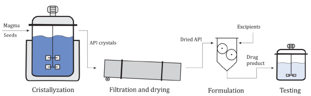
The method is tested with an in silico example for the crystallization and formulation of an active Pharmaceutical Ingredient (API). The API is derived from the reactor to the downstream processing steps. The solution containing the API is loaded to a crystallizer. The solid is then separated (via filtration and centrifugation) and dried. The purified crystals are then mixed with excipients and compacted into solid dosage form (i.e. tablets). The final product should be assessed in a dissolution test to verify that it fulfills a dissolution profile required by the Food and Drug Administration (FDA) of the Unites States. The overall process is shown in Fig. 2. The crystallizer operates in batch mode with an initial crystal seeding and following a temperature profile which is like the one proposed by Chung et al. (1999). The magma enters at saturation temperature and supersaturation is caused by the reduction of solubility due to steadily lowering the temperature. The temperature T at any given time t is set to perform the following profile:

(1)

In Eq. 1, T₀ and T_f are the initial and final temperature, t_f is the batch duration and γ is a process parameter of the temperature profile. The four optimization variables considered are closely related to the crystallizer´s operating conditions and are presented in Table 1. Other process variables are assumed fixed hereafter. They are summarized in Table 2.

Table 1. Optimization variables

Variable	Symbol
Mass of crystal seeds [kg]	M
Mean diameter of crystals [m]	d_m
Coefficient of variance [%]	CV
Temperature profile parameter	γ

Table 2. Fixed variables

Variable	Symbol	Value
Mass of magma [kg]	M_s	7570
Initial temperature [°C]	T₀	35
Final temperature [°C]	T_f	15
Batch duration [min]	t_f	240

Once the crystallization step is finished and the crystals are filtered and dried, the formulation step begins. The API is mixed with excipients and fractionated into tablets. A Gaussian error distribution with a 5% standard deviation in the API content is introduced in this processing step to simulate a source of intrinsic variability in the overall process of Fig. 2. Once the tablets have been obtained, they are tested in a dissolution assay. The test is performed in an agitated vessel that simulates the conditions in the human stomach (pH and temperature) as a proxy for bioavailability assessment. The tablets are subjected to grinding, then placed in the test vessel and the API concentration is measured at several sampling times. The concentration profile of the tablets is then compared with a reference profile. Two factors, f₁ and f₂, are calculated according to the Guidance for Industry FDA-1997-D-0187 provided by the FDA (1997):

(2)

(3)

In the Eqns. 2 and 3, Rp is the reference value and Cp is the test value for the percent dissolution of the API. In order to pass the test, f₁ should be less than 15% and f₂ should be higher than 50%. In this work, the reference profile for an API with a maximum content of 50 mg in 1 kg of solvent is shown in Table 3. Intrinsic variability of product formulation pose a challenge to repeatedly follow the reference profile.

C. In silico model

The crystallizer is simulated using the method of moments to calculate the main characteristics of the crystal’s size distribution. The equations for describing nucleation and growth rates are:

[#/m³.s] (4)

(5)

(6)

Table 3. Reference dissolution profile

Time [min]	Concentration [mg/kg]
0	0
15	4.92
30	9.48
45	13.70
60	17.57
75	21.05
90	24.34
120	30.03
180	38.80
240	45.30

In the Eq. 6, C is the API product concentration in the magma. The density of the API is 1050 kg/m³ and its solubility is a function of the crystallizer temperature:

(7)

Using these equations, the moments µ of the distributions can be calculated (Hulburt and Katz, 1964). The formulation step and the dissolution assay in the test vessel modify the moments according to a dilution factor f_d, that accounts for both the formulation and the change of volume from one tank to another:

(8)

The dilution factor is calculated as the API dissolution needed to achieve approximately 50 mg/kg in the test vessel (if dissolution is total), adding white noise of 5% to account for the intrinsic variability of the process. Finally, the moments are reduced while diluting. The dissolution rate and the API solubility in the new media are modeled by:

[m/s] (9)

(10)

III. RESULTS

The proposed Bayesian optimization method in Fig. 1 is applied as follows. For each operating policy tried, a crystallizer run is performed. The product crystals are dried, formulated and tested according to the dissolution assay. If the product successfully passes the dissolution assay (observation: +1), the run is considered successful, otherwise the experiment is considered a failure (observation: -1). An initial design of crystallization experiments to begin with, n₀, is defined using Latin Hypercube Sampling. Using the initial data set, the hyper-parameters of the GP metamodel are estimated. Then, the method proposes the next experiment by maximizing the acquisition function. The experiment is performed to generate additional data, which is used to update the GP metamodel. This is repeated until a maximum number n of experiments has been made. The trained GP for the one-class classification model is then used to solve the optimization problem that aims to maximize the probability of success of the process by finding the optimal operating policy for the crystallizer. Finally, the estimated optimal policy can be tried experimentally several times to estimate the true probability of success for the solution found. Typically, due to the intrinsic process variability this probability rarely is equal to 1.

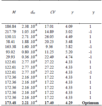
The initial and total number of experiments n₀and n are set to 7 and 15, respectively. The expected improvement for binary outcomes is chosen as the acquisition function. A summary of the experiments is presented in Table 4. After the initial set of experiments, the method tries an operating policy until one of the experiments doesn´t fulfill the end-use properties. After that, the method chooses a new operating policy and performs all the remaining experiments with it. Finally, an extra optimization step is carried out and the optimum is found to maximize the probability of success.

The values for the policy parameters are shown at the bottom of Table 4. The probability of success of the estimated optimal policy is approximately 100%. This is quite remarkable, given the low number of experiments performed and the complexity of the experimental optimization task: the probability of success of the operating policy must be obtained from binary responses of the experiments in a four-dimensional design space.

The evolution of the GP is shown in Fig. 3. The GP is initially trained with the first seven experiments, giving rise to the probability of success presented in Fig. 3(a). Only the first two elements of the operating policy (M and d_m) are shown, while the other two are fixed at the optimal values found for the sake of clarity.

The initial approximation in the form of a GP to the probability of success helps identifying a small region of operating conditions with higher probabilities of success, but the surface maximum is still flat, and more experiments are clearly needed. The GP is then increasingly updated with new experimental data and the final approximation to the probability of success after the last iteration is presented in Fig. 3(b). As can be seen there exists an optimum that is clearly distinguishable, with a maximum value for the success probability that is very close to 1. As exploitation of the generated knowledge is emphasized, the estimated maximum and nearby conditions will receive more attention and exploration vanishes.

It is noteworthy that the last five experiments of the available budget are made using the very same operating policy (see Table 4). This is due to bias introduced through hyper-parameters in the one-class classification model. In this work, to separate the positive class from the failure class, the following radial basis function is used:

(11)

Table 4. Optimization results

The hyper-parameter in Eq. 11 defines the characteristic length scale of the positive (success) class. The smaller the value of this parameter, the tighter (and smaller) the final ROI found by the Bayesian optimization algorithm in Fig. 1. Typically, to make enough room for exploration is better to choose initially high values for , and then profile down its values as more data is gathered. As a result, exploitation is favored over exploration as the budget for experimentation is being consumed. Eventually, gradual reduction of this hyper-parameter left almost no room for exploration. Note that the parameters of the operating policy must be conveniently scaled when defining the one-class classification model using the function in Eq. 11. The interested reader is referred to related works for details (Kemmler et al., 2013; Xiao et al., 2015).

A comparison of the performance of two operating policies is shown in Fig. 4. In Fig. 4(a), an arbitrarily chosen policy with parameters at the center of the design space is run 100 times. Run outcomes that do not fulfill the f₁or f₂ criterion are shown in dark blue, while the ones that do comply with dissolution specifications are shown in light blue. The optimal policy from Table 4 is shown in Fig. 4(b). As can be seen, all these runs made using the optimal policy fulfill the dissolution test criteria.

In order to test the robustness of the proposed approach, the algorithm was repeated 100 times. The average probability of success of the resulting operating policies is 93.9%, with 92 of the results having a probability of success of 80% or higher, and 72 of them having a

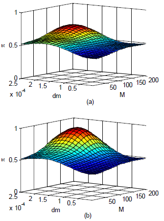
Figure 3: Projected approximations of the probability of success π over the ROI. (a) after the initial sampling and (b) after the optimal operating policy is found.

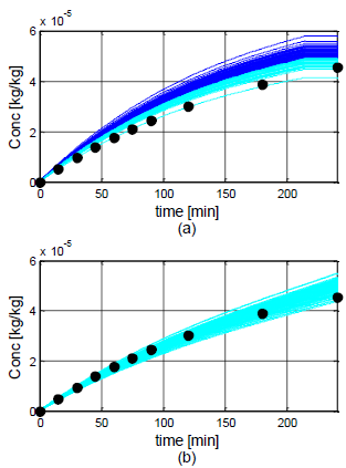
Figure 4: Dissolution profiles for (a) an arbitrary operating policy and (b) the optimal operating policy. Light blue lines are runs that successfully passed the test and dark blue lines are runs that did not. The target profile is shown with circles.

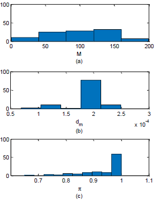
Figure 5: Histograms for the first (a) and second (b), policy parameters (M and d_m) of the optimal operating policy; (c) the probability of success for the optimal solution found.

probability of 90% or higher. Histograms of the first two policy parameters (M and d_m) of the optimal operating policies and their probability of success are presented in Fig. 5.

It is worth noting that the proposed experimental optimization method is quite robust despite just a few experiments were performed. If the total number of experiments were increased, the results will certainly improve. As an example, by doubling the number of experiments (from 15 to 30), the average probability of success of the optimal operating policies rises to 95.3%, and 96 of the results have a probability of success of 80% or higher, whereas 83 of them have a probability of 90% or higher. As can be expected, there is a trade-off between the cost of experimentation and the quality of the solution found.

IV. CONCLUSIONS

The applicability of Bayesian optimization in guaranteeing end-use product properties of crystallization processes has been discussed. Optimization results are promising bearing in mind the intrinsic level of variability considered in the formulation step, and that Bayesian optimization does not require a first-principles model of the crystallization and formulation processes. Also, Bayesian optimization takes advantage of any available data and imperfect models. Furthermore, the proposed approach is robust to both noise and outliers. Current research efforts are focused on considering multiple objectives and autonomous setting of hyper-parameters.

REFERENCES

Colombo, E., Luna, M.F. and Martínez, E.C. (2016). “Probability-Based Design of Experiments for Batch Process Optimization with End-Point Specifications,” Ind. Eng. Chem. Res., 55, 1254−1265.

Chung, S.H., Ma, D.L. and Braatz, R.D. (1999). “Optimal seeding in batch crystallization,” The Canadian journal of chemical engineering, 77, 590-596.

FDA. (1997). “Dissolution testing of immediate release solid oral dosage forms,” Food and Drug Administration, Center for Drug Evaluation and Research. Report FDA-1997-D-0187.

Fujiwara, M., Nagy, Z.K., Chew, J.W and Braatz, R.D. (2005). “First-principles and direct design approaches for the control of pharmaceutical crystallization,” J. Process Control,15, 493–504.

Gao, Z., Rohani, S., Gong, J. and Wang, J. (2017). “Recent Developments in the Crystallization Process: Toward the Pharmaceutical Industry,” Engineering, 3, 343–353.

Hurlburt, H. and Katz, S. (1964). “Some problems in particle technology,” Chem. Eng. Sci., 19, 555-574.

Kemmler, M., Rodner, E., Wacker, E.S. and Denzler, J. (2013). “One-class classification with Gaussian processes,” Pattern Recognition, 46, 3507–3518.

Lookman, T., Balachandran, P.V., Xue, D. and Ruihao, Y. (2019). “Active learning in materials science with emphasis on adaptive sampling using uncertainties for targeted design,” npj Computational Materials, 5, 1-21.

Lucke, M., Koudous, I., Sixt, M., Huter, M.J. and Strube, J. (2018). “Integrating crystallization with experimental model parameter determination and modeling into conceptual process design for the purification of complex feed mixtures,”

Chemical Engineering Research and Design, 133, 264–280.

Luna, M.F., and Martínez, E.C. (2018). “Sequential Bayesian Experimental Design for Process Optimization with Stochastic Binary Outcomes,” Computer-Aided Chemical Engineering, 43, 943-948.

Pruksawan, S., Lambard, G., Samitsu, S., Sodeyama, K. and Naito, M. (2019). “Prediction and optimization of epoxy adhesive strength from a small dataset through active learning,” Science and Technology of Advanced Materials, 20, 1010-1021.

Rasmussen, C.E. and Williams, C.K. (2006). Gaussian processes for machine learning, MIT Press, Cambridge, MA.

Shahriari, B., Swersky, K., Wang, Z., Adams, R.P. and de Freitas, N. (2016). “Taking the Human Out of the loop: A Review of Bayesian Optimization,” Proceedings of the IEEE, 104, 148-175.

Sun, J., Wang, F., Sui, Y., She, Z., Zhai, W., Wang, C. and Deng, Y. (2012). “Effect of particle size on solubility, dissolution rate, and oral bioavailability: evaluation using coenzyme Q₁₀ as naked nanocrystals,” International J. of Nanomedicine, 7, 5733–5744.

Talapatra, A., Boluki, S., Honarmandi, P., Solomou, A., Zhao, G., Ghoreishi, S.F., Molkeri, A., Allaire, D., Srivastava, A., Qian, X., Dougherty, E.R., Lagoudas, D.C. and Arróyave R., (2019). “Experiment Design Frameworks for Accelerated Discovery

of Targeted Materials Across Scales,” Frontiers in Materials, 6, 82.

Tesch, M., Schneider, J., and Choset, H. (2013). “Expensive Function Optimization with Stochastic Binary Outcomes,” J. of Machine Learning Research, 28, 1283-1291.

Wang, Y, Wang, C. and Powell, W. (2016). “The knowledge gradient for sequential decision making with stochastic binary feedbacks,” J. of Machine Learning Research, 48, 1138-1147.

Xiao, Y., Wang, H. and Xu, W. (2015). “Hyperparameter Selection for Gaussian Process One-Class Classification,” IEEE Trans. Neural Networks and Learning Systems, 26, 2182-2187.

Xue, D., Balachandran, P.V., Hogden, J., Theiler, J. Xue, D. and Lookman, T. (2016). “Accelerated search for materials with targeted properties by adaptive design,” Nature Communications, 7, 11241.

Received October 21, 2019

Sent to Subject Editor October 22, 2019

Accepted January 3, 2020

Recommended by Guest Editor: Carlos Apesteguia