Abstract-- In this work, we propose a modified version of the classical 20 nodes serendipity element for the dynamic analysis of doubly curved shells.

Instead of using the classical strain displacements relations, we propose to formulate the strain displacements relations in a general curvilinear coordinates. The main goal of the work is putting forward a 3D element, valid for general shell structures, which provides some desirable features like avoidance of locking and zero energy modes with decreasing thickness and good behaviour in dynamic analysis. Until now, most works are usually referred to shallow and thin shells. In this work the study of the vibrational frequencies of transverse oscillations of moderately thick shells by 3D elements for non shallow shells has been treated. We expose also different kinds of mass matrices and study a close variant of the classical lumped mass matrix.

Keywords-- Vibrations, finite elements, doubly curved shells, 3D elements.

I. INTRODUCTION

Vibration of shell structures is an interesting topic that has been manifested in many aspects of civil engineering and aeronautics. Shell structures are widely used in a variety of engineering applications and have the ability to withstand significant loads precisely because of its curvature which is responsible for providing additional resistance that differentiates them from other structural elements as plates.

Within the shell structures, the double curved ones, such as the hyperbolic paraboloid, the elliptic paraboloid or the velaroidal shells are significant structures in the field of civil engineering. Notwithstanding, the closed form solutions of the equilibrium equations are not generally possible to obtain them and it has to come to approximate methods Alhazza and Alhazza (2004).

The treaties of Leissa (1993) or Soedel (1993) are the first complete references to the dynamic analysis of plates and shells. These references study analytical solutions taking into account the equilibrium equations along orthogonal coordinate lines and usually in a membrane state.

General solutions of the equilibrium equations of shells in a general curvilinear system, taking into account the bending stresses, are a statically indeterminate problem so that it is necessary to look to approximate methods like the Finite Element Method.

FEM has been and is a very powerful tool for solving differential or integral equations in the context the structural calculation. A classical reference to this technique is the work of Zienkiewicz and Taylor (2000). Yang et al. (2004) show a good review of the Finite Element Methods for shell structures that have been developed since its inception back in the 60.

The dynamic study of doubly-curved shells is of particular interest because of its complex geometry, and the influence of the boundary conditions in the solution. Their approach by MEF has been collected in various works such as Liew and Lim (1995, 1996), Stavridis and Armenakas (1988) or Stavridis (1998). They use degenerated shell elements with several enhancements to avoid locking phenomenon but usually consider shallow shells and neglect shear deformation.

The reappearance of the three-dimensional finite elements in structural analysis is relatively recent and may come, in part, coupled with the large computing power of today's computers.

3D finite elements present some advantages against the most common degenerated shell elements, originally proposed by Ahmad et al (1970), since they include the possibility of using three-dimensional constitutive laws and do not use any kinematic assumption in deriving strain-displacement relations unlike shell theories.

However, most of the publications concerning to three-dimensional elements for the study of shells do with elements of 8 nodes. In order to relieve the well known problem of locking (membrane, shear and trapezoidal locking ) and zero energy modes, there have been proposed a lot of stabilization methods, hybrid models etc. See for example the work of Schwarze and Reese (2009) which has an interesting description of this type of elements.

In this paper we have preferred to use high order finite elements to address the problem. One advantage of higher order elements against these is that the appearance of the different lockings is much less significant. Specifically, we have tested the 20-node finite element (in its dynamic formulation) considering the strain displacements relations in a general curvilinear coordinates.

Details of the formulation and the results of some examples of interest are shown in the following sections.

II. PROBLEM FORMULATION USING 3D FINITE ELEMENTS. STIFFNESS MATRIX

For the reasons set out in the background, it has been chosen the 20 nodes serendipity element for the dynamic study of doubly curved shells. To define the shape functions, the isoparametric formulation is used in a coordinate system with origin at the center of the element (see Fig. 1).

In a compact form these equations can be written in the well known form:

(1)

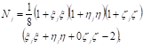
for corner nodes, j=1,….,8;

(2)

for mid-sides nodes, j=10,12,14,16.

(3)

for mid-sides nodes, j=9,11,13,15.

(4)

for mid-sides nodes j=17,18,19,20.

Using FEM, we have at least two coordinate systems: a Cartesian coordinate system (x,y,z) and other isoparametric system (x,h,z).

To solve the dynamic problem we have to find the stiffness matrix and the mass matrix of the element and after assembling the stiffness matrix and the mass matrix of the structure.

In matrix form we have to solve,

(5)

where K is the stiffness matrix and M the mass matrix of the structure.

This eigenvalue problem is well known and can be obtained from the Hamilton principle, for example. For more details it can be consulted Alhazza and Alhazza (2004).

The stiffness matrix [k_e] of the element in local coordinates can be expressed as, Zienkiewicz (2000):

(6)

where the matrix B is the relation between strains and displacements, det[J] is the determinant of the jacobian matrix and D is the constitutive matrix.

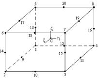
Figure 1: 20 nodes serendipity finite element.

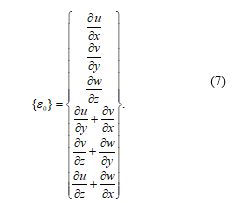
The relationship between strains and displacement {e₀} in the three-dimensional elasticity is:

If these strain - displacements relations are used, we would define the classical formulation of the 20 nodes serendipity element.

This last relationship can be written also,

If we take into account the relationship between the Cartesian coordinate system and the isoparametric one, we can express the derivatives of the displacements as functions of the isoparametric system,

where the elements G_ij are the components of the inverse of the jacobian matrix.

Following this last relation the matrix B can be written again as,

Finally the jacobian matrix can be written,

where (x_i, y_i, z_i) are the coordinates of the nodes of the element.

Until now, we have defined the classical formulation of the 20 nodes serendipity element. The behaviour of this element in static and dynamic analysis of shells has been proved satisfactory in several benchmarks. The coordinates of the nodes of the elements provide all the necessary information for defining the element and the shell (see Fig. 2).

In this work, a curvilinear local reference frame at the medium surface of the shell is preferred to work with, for an exact definition of the middle surface and to study the performance of the new element in dynamic shell analysis (see Fig. 3).

The first step to keep in mind is to recall the expression of the strains in a curvilinear system.

The expressions relating strains and displacements in curvilinear coordinates are (Rekach, 1978):

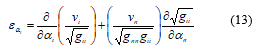
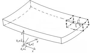
Figure 2: Cartesian Reference Frame and the isoparametric system.

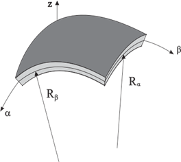
Figure 3: Curvilinear Local Reference Frame at the medium surface of the Shell

where e_a_i are the normal strains, g_ij are the engineering shear strains, g_ij are the components of the metric tensor referred to shell space, a_i are the intrinsic coordinates of the surface and v_i are the displacements. These well known expressions are written in terms of the physical components so we can directly interpolate the displacements.

Expanding these last relations we can obtain more comfortable expressions,

(15)

(16)

(17)

(18)

(19)

(20)

Or arranging these expressions in matrix form,

where displacements are interpolated, as usual, using the shape functions N_i.

Here we have made the approximation consisting in assimilating the metric tensor of the shell space g_ij to the reference shell surface a_ij. So the equations (15-20) take the form described in Eq. (21).

This assumption is only valid for moderately thick shells.

The constitutive equations in a general curvilinear coordinate system are quite different from the Cartesian ones and have the expression,

.(22)

Following Voight notation it can be expressed as a second order tensor in the form,

The corresponding relations with their physical components are,

, (24)

where g_a_b are the components of the metric tensor (Wempner and Talaslidis, 2002).

At this point, we only need to compute the differential volume element. Since we are working in a curvilinear local reference frame, we need to express it, if it is possible, as function of the curvilinear coordinates.

This relation is well known and can be consulted, for example, in Itskov (2009),

, (25)

where H and K are the mean and Gaussian curvature.

Let us note that all quantities present in the stiffness matrix of the element are functions of the thickness and the curvilinear coordinates.

III. MASS MATRIX OF THE 20 NODES SERENDIPITY ELEMENT. CONSISTENT AND LUMPED MASS MATRIX

In order to study the transverse frequencies of the structural element concerned by the finite element method, we must develop the mass matrix of the element. When we take the same shape functions for interpolating the geometry of the element as to discretize the kinetic energy, we have the so-called consistent mass matrix of the finite element.

If we develop this expression, we find:

Or in matrix form,

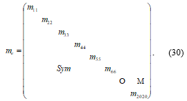
Another possibility in this regard is to construct the lumped mass matrix. This mass matrix is traditionally less effective than consistent mass matrix but more efficient to be a square diagonal matrix. The mass of the element is concentrated uniformly in all nodes.

(29)

where a,b and c are the finite element dimensions.

In this work, we have opted for a more rational distribution of the masses at the nodes taking into account the geometry of the element and the distribution of nodes in it.

If L_x, L_h and L_z are the dimensions of the element according to isoparametric coordinates of the element, surface mapping and lengths to calculate volume and mass associated with the nodes of the element can be drawn considering the Figs. 4 and 5.

Figure 4: Distribution of areas in the upper and lower surface of the 20 nodes element

Figure 5: Distribution of areas in the medium surface of the 20 nodes element.

Figure 6: Hp- Shell. Discretization by finite elements.

So that the masses distribution at the nodes is not uniform but is made taking into account geometrical and symmetry considerations of the contribution of each node to the mass matrix of the element.

Since, the mass matrix adopts the form

IV. RESULTS

To test the goodness of this work we have previously tested the modified version of the 20 nodes serendipity element with the results obtained by other authors with the hyperbolic paraboloid shells, whose solutions are known according to the works of Narita and Leissa (1984), Chakravorty and Bandyopadhyay (1995) and Chakravorty et al. (1995), but they used shell elements. The hyperbolic paraboloid test is quite demanding both surface type (doubly curved shell) and the boundary conditions.

The data we have used for the example are: hyperbolic paraboloid with curved edges, square planform 1´1 m side, constant thickness of 0.01 m, equal radii of curvature and opposite in value R=2m, Young modulus E=10.92´10⁶ N/m², Poisson's ratio 0.30, density= 100 kg/m³, subjected to a uniformly distributed load of 20 kN/m² and clamped along the four edges. In all cases we have used the lumped mass matrix proposed by the authors.

The frequency associated with the first mode of vibration of the hyperbolic paraboloid according the new formulation is 17, 23rad / s. The results obtained by the above-named authors are:

· Narita-Leissa: 17.16 rad/s

· Chakravorty : 17.25 rad/s

Displacements associated with the second and third vibration modes, which have not been found in the literature, are depicted in the following figures (see Figs. 7 and 8):

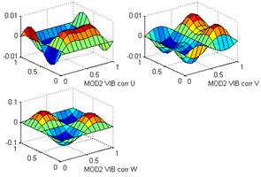
Figure7: Displacements (u,v,w) associated with the second vibration mode of the hyperbolic paraboloid. Modified version of the 20 nodes serendipity element.

Figure 8: Displacements (u,v,w) associated with the third vibration mode of the hyperbolic paraboloid. Modified version of the 20 nodes serendipity element.

In order to compare high order modes of vibration, we compare the results with the work of Liew and Lim (1996).

The results are presented for the nondimensional frequency parameter λ given by,

The natural frequencies w, the rectangular planform Lengths (a,b), and the shell thickness h are represented in this last equation.

For simply supported hyperbolic paraboloid shell with square planform, the results are compared for the first, fourth and eight vibration modes given in the work of Liew and Lim (1996).

In this case we take, v=0.3, a/b=1, b/h=100. The results are shown in the Table 1.

As we can see, there exists a good agreement between the results if the shallowness ratio is small. But if the shallowness ratio increases, the differences become greater.

The results obtained with the classical formulation of the 20 nodes element, is closer to the results of the work of Liew and Lim (1996).

In order to compare the results with moderately thick shells, we use the parameter l’, given by

Table 1: Comparison of frequency parameter λ for simply supported thin hyperbolic paraboloidal shells and various values for b/Ry and Ry/Rx. Modified version of the 20 nodes serendipity element.

b/ Ry	Ry/ Rx	Mode sequence number	1	4	8
0.1	1	Liew and Lim (1996)	42.688	83.136	130.86
	1	Present	42.681	84.062	133.80
	05	Liew and Lim (1996)	36.713	81.902	130.71
	05	Present	36.715	82.887	133.52
0.3	1	Liew and Lim (1996)	104.02	110.78	150.76
	1	Present	103.42	110.79	151.22
	0.5	Liew and Lim (1996)	75.152	102.10	148.35
	0.5	Present	75.082	102.25	148.99
0.5	1	Liew and Lim (1996)	148.74	159.39	198.54
	1	Present	145.62	160.34	196.79
	0.5	Liew and Lim (1996)	105.48	136.48	177.97
	0.5	Present	104.66	137.11	178.99

Table2: Comparison of the frequency parameter λ’ for simply supported moderately thick hyperbolic paraboloidal shells. Comparison of the results obtained with the Classical Formulation (C.F.) and the modified version of the 20 nodes serendipity element, new formulation, (N.F.).

b/ Ry	Ry/ Rx	Mode sequence number	1	4	8
0.1	1	N.F.	0.571	2.072	3.233
	1	C. F.	0.575	2.064	3.164
	0.5	N.F.	0.568	2.079	3.237
	0.5	C. F.	0.552	1.998	3.081
0.3	1	N.F.	0.657	2.072	3.220
	1	C. F.	0.655	2.059	3.175
	0.5	N.F.	0.623	2.072	3.227
	0.5	C. F.	0.636	2.054	3. 192
0.5	1	N.F.	0.784	2.051	3.182
	1	C. F.	0. 762	1.998	3.126
	0.5	N.F.	0.722	2.066	3.221
	0.5	C. F.	0.718	2.042	3.183

In this case we take, v=0.3, a/b=1, b/h=10. We have analyzed the results with both versions of the 20 nodes serendipity element, the classical formulation and the new formulation. Similar conclusions can be derived regarding the previous analysis. It has to be taken into consideration that the effect of the shear deformation has not been neglected. The results are shown in the Table 2.

To conclude our work, we have also studied the natural frequencies of other kind of surfaces like the cylindrical shell and the spherical shell. The boundary conditions are also simply supported shell. The results with the new finite element are compared again with the analysis of Liew and Lim (1996) are shown in Table 3, for v=0.3, a/b=1, b/h=100.

Given these results, the efficiency of both elements is very high. However we appreciate that the results obtained with classical formulation are closer to the shallow shell theory whilst the new formulation is closer to the deep shell theory. For simply supported shells it is observed that lower and higher frequencies vary linearly with the shallowness ratio.

V. CONCLUSIONS AND FUTURE WORK

In this work, we have studied the vibrations of doubly curved shells with 3D elements with a modified version of the classical 20 nodes serendipity element, considering the strain-displacement relations in a curvilinear system tangent to the middle surface of the shell.

The exact knowledge of the metric tensor of the middle surface as well as other geometric quantities provide excellent results for non-shallow doubly curved shells. Besides, the problems associated with low order displacements 3D finite elements, shear and trapezoidal locking, which predict spurious shear and normal stresses, are circumvented.

A rational approach to the lumped mass matrix has been used, taking into account the geometry of the element. New results for moderately thick shells have been obtained and important conclusions about the variation of the frequencies´ with respect to the shallowness ratio have been deduced.

Results for the vibrations of other doubly curved shells with different boundary conditions and the analysis of the sensitivity of the formulation to element distortions will be presented in a future work due to its extension.

Table3: Comparison of the frequency parameter λ for simply supported thin cylindrical and spherical shell. Comparison of the results obtained with the work of Liew and Lim (1996) and the new formulation of the 20 nodes serendipity element.

b/ Ry	Ry/ Rx	Mode sequence number	1	4	8
0.1	0	Liew and Lim (1996)	36.841	82.302	131.11
	0	Present	36.021	82.415	133.76
	0.5	Liew and Lim (1996)	43.027	84.316	132.05
	0.5	Present	42.229	85.163	134.28
	1	Liew and Lim (1996)	53.049	87.829	133.51
	1	Present	52.693	88.930	134.72
0.3	0	Liew and Lim (1996)	66.574	104.95	151.49
	0	Present	66.157	106.10	153.64
	0.5	Liew and Lim (1996)	86.927	118.41	158.69
	0.5	Present	86.001	118.83	160.24
	1	Liew and Lim (1996)	121.99	139.21	169.68
	1	Present	119.54	141.58	170.55
0.5	0	Liew and Lim (1996)	88.431	140.07	182.95
	0	Present	87.984	143.01	183.63
	0.5	Liew and Lim (1996)	127.81	165.19	200.99
	0.5	Present	128.54	167.73	202.38
	1	Liew and Lim (1996)	188.59	201.27	239.87
	1	Present	200.63	202.46	241.51

REFERENCES

Ahmad, S., B. Irons and O.C. Zienkiewicz, “Analysis of thick and thin shell structures by curved finite elements,” International Journal for Numerical Methods in Engineering, 2, 419-451 (1970).

Alhazza, K. and A. Alhazza, “A review of the vibrations of plates and shells,” The Shock and Vibration Digest, 36, 377–395 (2004).

Chakravorty, D. and J. Bandyopadhyay, “On the free vibration of shallow shells,” Journal of Sound and Vibration, 185, 673–684 (1995).

Chakravorty, D., J.N. Bandyopadhyay and P. K. Sinha, “Free vibration of point-supported laminated doubly curved shells–A finite element approach,” Comput Struct, 54, 191–198 (1995).

Itskov, M., Tensor Algebra and Tensor Analysis for Engineers: With Applications to Continuum Mechanics, Springer (2009).

Leissa, A.W., Vibration of Shells, Acoustical Society of America, Sewickly (1993).

Liew, K. and C. Lim, “Vibratory behaviour of doubly curved shallow shells of curvilinear planform,” Journal of Engineering Mechanics, 121, 1277–1283 (1995).

Liew, K. and C. Lim, “Vibration of doubly-curved shallow shells,” Acta Mechanica, 114, 95–119 (1996).

Narita, Y. and A.W. Leissa, “Vibrations of corner point supported shallow shells of rectangular planform,” Earthquake Engineering and Structural Dynamics, 12, 651–661 (1984).

Rekach, V.G., Manual of the theory of Elasticity, Mir Moscow (1978).

Schwarze, M. and S. Reese, “A reduced integration solid-shell finite element based on the EAS and the ANS concept-Geometrically linear problems,” International Journal for Numerical Methods in Engineering, 80, 1322-1355 (2009).

Soedel, W., Vibrations of Shells and Plates, Marcel Dekker, New York (1993).

Stavridis, L., “Dynamic analysis of shallow shells of rectangular base,” Journal of Sound and Vibration, 218, 861–882 (1998).

Stavridis, L. and A. Armenakas, “Analysis of shallow shells with rectangular projection,” Journal of Engineering Mechanics, 114, 943–952 (1988).

Yang, H., S. Saigal, A. Masud and R. Kapania, “A survey of recent shell finite elements,” International Journal for Numerical Methods in Engineering, 4, 101–127 (2004).

Wempner, G. and D. Talaslidis, Mechanics of Solids and Shells: Theories and Approximations, CRC Press (2002).

Zienkiewicz, O.C. and L.R. Taylor, The Finite Element Method. Solid Mechanics, Wiley (2000).

Received: April 11, 2015.

Sent to Subject Editor: November 30 2015.

Accepted: April 13, 2016.

Recommended by Subject Editor: Walter Tuckart